Kestrel Command

A Kestrel command describes a Hunt Step in one of the five categories:

1. Retrieval: GET, FIND, NEW.

2. Transformation: SORT, GROUP.

3. Enrichment: APPLY.

4. Inspection: INFO, DISP, DESCRIBE.

5. Flow-control: SAVE, LOAD, ASSIGN, MERGE, JOIN.

To achieve Composable Hunt Flow and allow threat hunters to compose hunt flow freely, the input and output of any Kestrel command are defined as follows:

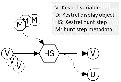
A command takes in one or more variables and maybe some metadata, for example, the path of a data source, the attributes to display, or the arguments to analytics. Then, the command can either yield nothing, a variable, a display object, or both a variable and a display object.

• As illustrated in the figure of Composable Hunt Flow, Kestrel variables consumed and yielded by commands play the key role to connect different hunt steps (commands) into hunt flows.

• A display object is something to be displayed by a Kestrel front end, for example, a Jupyter Notebook. It is not consumed by any of the following hunt steps. It only presents information from a hunt step to the user, such as a tabular display of entities in a variable, or an interactive visualization of entities.

Command	Take Variable	Take Metadata	Yield Variable	Yield Display
GET	no	yes	yes	no
FIND	yes	yes	yes	no
NEW	no	data	yes	no
APPLY	yes (multiple)	yes	no (update)	maybe
INFO	yes	no	no	yes
DISP	yes	maybe	no	yes
DESCRIBE	yes	no	no	yes
SORT	yes	yes	yes	no
GROUP	yes	yes	yes	no
SAVE	yes	yes	no	no
LOAD	no	yes	yes	no
ASSIGN	yes	no	yes	no
MERGE	yes (two)	no	yes	no
JOIN	yes (two)	yes	yes	no

GET

The command GET is a retrieval hunt step to match a Extended Centered Graph Pattern (ECGP) defined in Graph Pattern and Matching against a pool of entities and return a list of homogeneous entities (a subset of entities in the pool satisfying the pattern).

Syntax

returned_variable = GET returned_entity_type [FROM entity_pool] WHERE ecgp [time_range] [LIMIT limit]

• The returned_entity_type is specified right after the keyword GET.

• The entity_pool is the pool of entities from which to retrieve data:

  • The pool can be a data source, which has different types of entities in the records yielded/stored in that data source. For example, a data source could be a data lake where monitored logs are stored, an EDR, a firewall, an IDS, a proxy server, or a SIEM system. entity_pool is the identifier of the data source, e.g.:

    • stixshifter://host101: EDR on host 101 via STIX-shifter Data Source Interface.

    • https://a.com/b.json: sealed telemetry data in a STIX bundle.

  • The pool can also be an existing Kestrel variable (all entities of the same type in that variable). In this case, entity_pool is the variable name.

  • In general, the FROM clause is required for a GET command. There is one exception: the Kestrel runtime remembers the last data source used in a GET command in a hunting session. If there already are GET commands with data source (not variable) as entity_pool executed in the session, and the user wants to write a new GET command with the same data source, the FROM clause can be omitted (see examples in the next subsection). Note if the front-end allows out-of-order execution, e.g., executing the first cell after the second cell in Jupyter Notebook, Kestrel runtime will treat the GET command in the first (not the second) cell as the last GET command in this session.

• The ecgp in the WHERE clause describe the returned entities. Check out Graph Pattern and Matching to learn ECGP and how to write a pattern.

• The time_range is described in Time Range with both absolute and relative time range syntax avaliable. This is optional, and Kestrel will try to specify a time range for the pattern with the following order (smaller number means higher priority):

  1. User-specified time range using the Time Range syntax if provided.

  2. Time range from Kestrel variables in ECGP if exist.

  3. STIX-shifter connector default time range, e.g., last five minutes, if the STIX-shifter Data Source Interface is used.

  4. No time range specified for the generated query to a data source.

• The limit is an optional argument that specifies the number of records to be returned by the GET query. In the current implementation, Kestrel will return limit observed-data records. The number of returned_entity_type records returned could be different because it depends on how many returned_entity_type records are included in the observed-data dataset.

Learn how to setup data sources via existing Kestrel data source interfaces such as STIX-shifter Data Source Interface at Connect to Data Sources. Read Kestrel Interfaces to understand more about the abstraction of interface and how to develop new data source interfaces.

Examples

# get processes from host101 which has a parent process with name 'abc.exe'
procs = GET process FROM stixshifter://host101 WHERE parent_ref.name = 'abc.exe'
        START 2021-05-06T00:00:00Z STOP 2021-05-07T00:00:00Z

# get files from a sealed STIX bundle with hash 'dbfcdd3a1ef5186a3e098332b499070a'
# Kestrel allows to write a command in multiple lines
binx = GET file
       FROM https://a.com/b.json
       WHERE hashes.MD5 = 'dbfcdd3a1ef5186a3e098332b499070a'
       START 2021-05-06T00:00:00Z STOP 2021-05-07T00:00:00Z

# get processes from the above procs variable with pid 10578 and name 'xyz'
# usually no time range is used when the entity pool is a varible
procs2 = GET process FROM procs WHERE pid = 10578 AND name = 'xyz'

# refer to another Kestrel variable in the WHERE clause (ECGP)
# Kestrel will infer time range from `procs2`; users can override it by providing one
procs3 = GET process FROM procs WHERE pid = procs2.pid

# omitting the FROM clause, which will be desugarred as 'FROM https://a.com/b.json'
procs4 = GET process WHERE pid = 1234
         START 2021-05-06T00:00:00Z STOP 2021-05-07T00:00:00Z

FIND

The command FIND is a retrieval hunt step to return entities connected to a given list of entities.

Syntax

returned_variable = FIND returned_entity_type RELATIONFROM input_variable [WHERE ecgp] [time_range] [LIMIT limit]

Kestrel defines two categories of relations: 5 sepcific relations and 1 generic relation. Specifc relations are directed, and the generic relation is non-directed. Details in the figure:

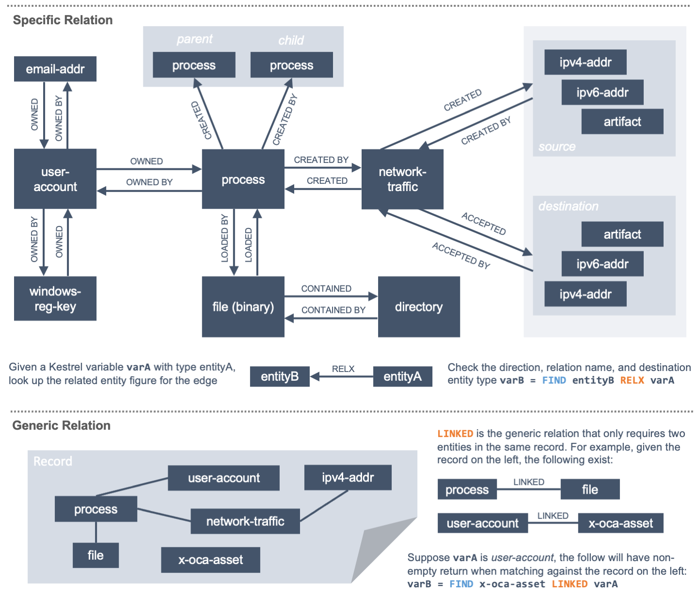
The Kestrel relation is largely based on the standard STIX data model, e.g., _ref in STIX 2.0 and SRO in STIX 2.1. While STIX is extensible and a data source can bring their own mappings of custom relations, Kestrel only implements the relation supported in standard STIX to ensure its commonality. The good part is this automatically works on all stix-shifter connectors, which mostly follow standard STIX. The bad part is standard STIX does not define file read/write/create/delete by process, so these specific relations are missing currently. Users can use the generic relation to find a superset of related entities as a partial solution.

Examples

# find parent processes of processes in procs
parent_procs = FIND process CREATED procs

# find child processes of processes in procs
parent_procs = FIND process CREATED BY procs

# find network-traffic associated with processes in procs
nt = FIND network-traffic CREATED BY procs

# find processes associated with network-traffic in nt
ntprocs = FIND process CREATED network-traffic

# find source IP addresses in nt
src_ip = FIND ipv4-addr CREATED nt

# find destination IP addresses in nt
src_ip = FIND ipv4-addr ACCEPTED nt

# find both source and destination IP addresses in nt
src_ip = FIND ipv4-addr LINKED nt

# find network-traffic which have source IP src_ip
ntspecial = FIND network-traffic CREATED BY src_ip

Limited ECGP in FIND

The WHERE clause in FIND is an optional component to add constraints when generating low-level queries to data sources. Similar to the GET command, an ECGP is used in the WHERE clause of FIND. However, one only needs to write the extended subgraph component in the ECGP in FIND. If there is a centered subgraph component in the ECGP in FIND, it will be discarded/abandoned in the evaluation, a.k.a., when Kestrel generates low-level queries. The design rationale:

1. In GET, the WHERE clause is the only place to describe constraints for the return variable.

2. In FIND, the major constraint for the return variable is provided by the relation already. The return variable connected from the input variable by a given relation is, in essence, an one-hop centered subgraph.

3. If the ECGP has centered subgraph component, it could conflict with the generated one-hop centered subgraph in the second point. So Kestrel discards the centered subgraph component in ECGP in FIND if exist.

4. The extended subgraph does not conflict with the relation in FIND, and it could give extra constraints to avoid unnecessary computation/transmision, so it is included in the low-level queries generated to the data source.

For example, the following is a fully valid FIND with ECGP:

# find parent processes of processes in procs
#
# the added WHERE clause limits the search to be performed against endpoint101
#
# if there are other endpoints data in the data source (used to get `procs`),
# they will not be matched against
#
# assume the process identifier such as pid is reused across endpoints,
# this will reduce false positives and avoid unnecessary computation/transmision
#
parent_procs_ww = FIND process CREATED procs
                  WHERE x-oca-asset:hostname = 'endpoint101'

If a user writes the following, it actually results the same as the above example:

# the centered subgraph `process:name = 'bash'` in the following command
# will be abandoned when executing, resulting parent_procs_ww2 == parent_procs_ww
parent_procs_ww2 = FIND process CREATED procs
                   WHERE name = 'bash' AND x-oca-asset:hostname = 'endpoint101'

If the user wants to match parent processes that are only bash, he/she needs a two-step huntflow:

parent_procs_ww = FIND process CREATED procs
                  WHERE x-oca-asset:hostname = 'endpoint101'

parent_procs_bash = parent_procs_ww WHERE name = 'bash'

Time Range in FIND

The time_range is optional—Kestrel will infer time range from the input_variable similarly to the time inference in Referring to a Variable in an ECGP. The user needs to provide a Time Range only if he/she wants to override the inferred time range from input_variable.

Example of overrode time range: A service process run on a host for several days. The record of the process creation/forking happends on day 1, while most of its activities happend on day 4-5. A hunt of the process starts covering day 4-5 with a few GET. When the hunter wants to FIND the parent process of the service process, he/she retrieves nothing if he/she does not specify a time range (the process creation record is beside the inferred time range: day 4-5). The hunter can broaden and override the time range in the FIND command with a specified Time Range to finally retrieve the parent process. No one (the hunter or Kestrel) knows when the process is created/forked, so it may take a few trial and error before the hunter broadens the time range in FIND large enough to retrieve the parent process. Sketches of the huntbook:

# some early hunt steps
nt = GET network-traffic
     FROM stixshifter://edp
     WHERE dst_ref.value = '10.10.30.1'
     LAST 5 DAY

# it is OK to write this FIND without time range
# which only search for the time range of `nt` for any records of `p1`
p1 = FIND process CREATED nt

# then, `pp1` will be empty (if the process is created 10 days ago)
# - `p1` is assocaited with time range inferred from `nt` (last 5 days)
# - no record in the last 5 days is about process creation of `p1`
# - so Kestrel cannot grab anything about the parent process of `p1`
pp1 = FIND process CREATED p1

# alternatively, override the time range when retrieving data for `p2`
# telling Kestrel to search for all `p2` records within the last 10 days
p2 = FIND process CREATED nt LAST 10 DAY

# now the parent process will be discovered
pp2 = FIND process CREATED p2

Limit in FIND

The limit is an optional argument that specifies the number of records to be returned by the FIND query. In the current implementation, Kestrel will return limit observed-data records. The number of returned_entity_type records returned could be different because it depends on how many returned_entity_type records are included in the observed-data dataset.

Relation With GET

Both FIND and GET are retrieval hunt steps. GET is the most fundamental retrieval hunt step. And FIND provides a layer of abstraction to retrieve connected entities more easily than using the raw GET for this, that is, FIND can be replaced by GET in theory with some knowledge of how to hunt. Kestrel tries to focus threat hunters on what to hunt and automate the generation of how to hunt (see What is Kestrel?). Finding connected entities requires knowledge on how the underlying records are connected, and Kestrel resolves the how for users with the command FIND.

In theory, you can replace FIND with GET and a parameterized STIX pattern when knowing how the underlying records are connected. In reality, this is not possible with STIX pattern in GET.

• The dereference of connection varies from one data source to another. The connection may be recorded as a reference attribute in a record like the *_ref attributes in STIX 2.0. It can also be recorded via a hidden object like the SRO object in STIX 2.1.

• STIX does not maintain entity identification across record (STIX observation). It is unclear how to refer to an existing entity in a new STIX pattern, e.g., is the process from the forking and networking records/events/observations the same process even with the same pid? Kestrel uses comprehensive Entity Identification logic to identify entities across record.

NEW

The command NEW is a special retrieval hunt step to create entities directly from given data.

Syntax

returned_variable = NEW [returned_entity_type] data

The given data can either be:

• A list of string [str]. If this is used, returned_entity_type is required. Kestrel runtime creates the list of entities based on the return type. Each entity will have one initial attribute.

  • The name of the attribute is decided by the returned type.

    Return Entity Type	Initial Attribute
    process	name
    file	name
    mutex	name
    software	name
    user-account	user_id
    directory	path
    autonomous-system	number
    windows-registry-key	key
    x509-certificate	serial_number

  • The number of entities is the length of the given list of string.

  • The value of the initial attribute of each entity is the string in the given data.

• A list of dictionaries [{str: str}]. All dictionaries should share the same set of keys, which are attributes of the entities. If type is not provided as a key, returned_entity_type is required.

The given data should follow JSON format, for example, using double quotes around a string. This is different from a string in STIX pattern, which is surrounded by single quotes.

Examples

# create a list of processes with their names
newprocs = NEW process ["cmd.exe", "explorer.exe", "google-chrome.exe"]

# create a list of processes with a list of dictionaries
newvar = NEW [ {"type": "process", "name": "cmd.exe", "pid": "123"}
             , {"type": "process", "name": "explorer.exe", "pid": "99"}
             ]

# return entity type is required if not a key in the data
newvar2 = NEW process [ {"name": "abc.exe", "pid": "1234"}
                      , {"name": "ie.exe", "pid": "10"}
                      ]

APPLY

The command APPLY is an enrichment hunt step to compute and add attributes to Kestrel variables, as well as generating visualization objects. This is called enrichment since the results of an external computation is merged back to a huntflow as new/updated attributes of the returned entities. The external computation, a.k.a., an analytics in Kestrel, can perform detection, threat intelligence enrichment, anomaly detection, clustering, visualization, or any computation in any language. This mechanism makes the APPLY command a foreign language interface to Kestrel.

Syntax

APPLY analytics_identifier ON var1, var2, ... WITH x=abc, y=[1,2,3], z=varx.pid

• Input: The command takes in one or multiple Kestrel variables such as var1, var2.

• Arguments: The WITH clause specifies arguments used in the analytics.

  • Arguments are provided in key-value pairs, split by ,.

  • A value is either a literal string, quoted string (with escaped characters), list, or nested list.

  • A list in a value is specified/wrapped by either () or [].

  • A nested list in value will be flattened before passing to the analytics.

  • A value can contain references to Kestrel variables. Like variable reference in ECGP, an attribute of entities needs to be specified when a Kestrel variable is referred. Kestrel will de-reference the attribute/variable, e.g., z=varx.pid will enumerate all pid of variable varx, which may be unfolded to [4, 108, 8716], and the final argument is z=[4,108,8716] when passed to the analytics.

• Execution: The command executes the analytics specified by analytics_identifier like docker://ip_domain_enrichment or python://pin_ip_on_map.

  There is no limitation for what an analytics could do besides the input and output specified by its corresponding Kestrel analytics interface (see Kestrel Interfaces). An analytics could run entirely locally and then just do a table lookup. It could reach out to the Internet like the VirusTotal service. It could perform real-time behavior analysis of binary samples. Based on specific analytics interfaces, some analytics can run entirely in the cloud, and the interface harvests the results to local Kestrel runtime.

  Threat hunters can quickly wrap an existing security program/module into a Kestrel analytics. For example, creating a Kestrel analytics as a docker container and utilizing the existing Kestrel Docker Analytics Interface (check Docker Analytics Interface). You can also easily develop new analytics interfaces to provide special running environments (check Kestrel Analytics Interface).

  Check Setup Kestrel Analytics to learn more about setup/using Kestrel analytics.

• Output: The executed analytics could yield either or both of (a) data for variable updates, or (b) a display object. The APPLY command passes the impacts to the Kestrel session:

  • Updating variable(s): The most common enrichment is adding/updating attributes to input variables (existing entities). The attributes can be, yet not limited to:

    • Detection results: The analytics performs threat detection on the given entities. The results can be any scalar values such as strings, integers, or floats. For example, malware labels and their families could be strings, suspicious scores could be integers, and likelihood could be floats. Numerical data can be used by later Kestrel commands such as SORT. Any new attributes can be used in the WHERE clause of the following GET commands to pick a subset of entities.

    • Threat Intelligence (TI) information: Commonly known as TI enrichment, for example, Indicator of Comprise (IoC) tags.

    • Generic information: The analytics can add generic information that is not TI-specific, such as adding software description as new attributes to software entities based on their name attributes.

  • Kestrel display object: An analytics can also yield a display object for the front end to show. Visualization analytics yield such data such as our python://pin_ip_on_map analytics that looks up the geolocation of IP addresses in network-traffic or ipv4-addr entities and pin them on a map, which can be shown in Jupyter Notebooks.

• There is no new return variable from the command.

Community-Contributed Kestrel Analytics

The community-contributed Kestrel analytics are in the kestrel-analytics repo, covering detection, TI enrichment, information lookup, visualization, machine learning, and more. They can be invoked either through the Docker or the Python analytics interface. More in Setup Kestrel Analytics.

Examples

# A visualization analytics:
# Finding the geolocation of IPs in network traffic and pin them on a map
nt = GET network-traffic FROM stixshifter://idsX WHERE dst_port = 80
APPLY docker://pin_ip ON nt

# A beaconing detection analytics:
# a new attribute "x_beaconing_flag" is added to the input variable
APPLY docker://beaconing_detection ON nt

# A suspicious process scoring analytics:
# a new attribute "x_suspiciousness" is added to the input variable
procs = GET process FROM stixshifter://server101 WHERE parent_ref.name = 'bash'
APPLY docker://susp_proc_scoring on procs
# sort the processes
procs_desc = SORT procs BY x_suspiciousness DESC
# get the most suspicous ones
procs_sus = GET process FROM procs WHERE x_suspiciousness > 0.9

# A domain name lookup analytics:
# a new attribute "x_domain_name" is added to the input variable for its dest IPs
APPLY docker://domain_name_enrichment ON nt

INFO

The command INFO is an inspection hunt step to show details of a Kestrel variable.

Syntax

INFO varx

The command shows the following information of a variable:

• Entity type

• Number of entities

• Number of records

• Entity attributes

• Indirect attributes

• Customized attributes

• Birth command

• Associated datasource

• Dependent variables

The attribute names are especially useful for users to construct DISP command with ATTR clause.

Examples

# showing information like attributes and how many entities in a variable
nt = GET network-traffic FROM stixshifter://idsX WHERE dst_port = 80
INFO nt

DISP

The command DISP is an inspection hunt step to print attribute values of entities in a Kestrel variable. The command returns a tabular display object to a front end, for example, Jupyter Notebook.

Syntax

DISP [TIMESTAMPED(varx)|varx]
     [WHERE ecgp]
     [ATTR attribute1, attribute2, ...]
     [SORT BY attibute [ASC|DESC]]
     [LIMIT l [OFFSET n]]

• The optional transform TIMESTAMPED retrieves the first_observed timestamped for each observation of each entity in varx. More is discussed in Variable Transforms.

• The optional clause WHERE specifies an ECGP (defined in Graph Pattern and Matching) as filter. Only the centered subgraph component (not extended subgraph) of the ECGP will be processed for the DISP command.

• The optional clause ATTR specifies which list of attributes you would like to print. If omitted, Kestrel will output all attributes.

• The optional clause SORT BY specifies which attribute to use to to order the entities to print.

• The optional clause LIMIT specifies an upper limit on the number of entities to print.

• The command deduplicates rows. All rows in the display object are distinct.

• The command goes through all records/logs in the local storage about entities in the variable. Some records may miss attributes that other records have, and it is common to see empty fields in the table printed.

• If you are not familiar with the data, you can use INFO to list all attributes and pick up some attributes to write the DISP command and ATTR clause.

Examples

# display <source IP, source port, destination IP, destination port>
nt = GET network-traffic FROM stixshifter://idsX WHERE dst_port = 80
DISP nt ATTR src_ref.value, src_port, dst_ref.value, dst_port

# display process pid, name, and command line
procs = GET process FROM stixshifter://edrA WHERE parent_ref.name = 'bash'
DISP procs ATTR pid, name, command_line

# display the timestamps from observations of those processes:
DISP TIMESTAMPED(procs) ATTR pid, name, command_line

DESCRIBE

The command DESCRIBE is an inspection hunt step to show descriptive statistics of a Kestrel variable attribute.

Syntax

DESCRIBE varx.attr

The command shows the following information of an numeric attribute:

• count: the number of non-NULL values

• mean: the average value

• min: the minimum value

• max: the maximum value

The command shows the following information of other attributes:

• count: the number of non-NULL values

• unique: the number of unique values

• top: the most freqently occurring value

• freq: the number of occurrences of the top value

Examples

# showing information like unique count of src_port
nt = GET network-traffic FROM stixshifter://idsX WHERE dst_port = 80
DESCRIBE nt.src_port

SORT

The command SORT is a transformation hunt step to reorder entities in a Kestrel variable and output the same set of entities with the new order to a new variable. While the SORT clause in DISP only alters the order of entities once for the display, the SORT command reorders the entities (in a variable) in the store of the session, thus all follow-up commands using the variable will see entities in the updated order. Most Kestrel commands are order insensitive, yet an entity-order-sensitive analytics can be developed and invoked by APPLY.

Syntax

newvar = SORT varx BY attribute [ASC|DESC]

• attribute is an attribute name like pid or x_suspicious_score (after running the Suspicious Process Scoring analytics) if varx is process.

• By default, data will be sorted by descending order. The user can specify the direction explicitly such as ASC: ascending order.

Examples

# get network traffic and sort them by their destination port
nt = GET network-traffic FROM stixshifter://idsX WHERE dst_ref_value = '1.2.3.4'
ntx = SORT nt BY dst_port ASC

# display all destination port and now it is easy to check important ports
DISP ntx ATTR dst_port

GROUP

The command GROUP is a transformation hunt step to group entities based on one or more attributes as well as computing aggregated attributes for the aggregated entities.

Syntax

aggr_var = GROUP varx BY attr1, attr2... [WITH aggr_fun(attr3) [AS alias], ...]
aggr_var = GROUP varx BY BIN(attr, bin_size [time unit])... [WITH aggr_fun(attr3) [AS alias], ...]

• Numerical and timestamp attributes may be “binned” or “bucketed” using the BIN function. This function takes 2 arguments: an attribute, and an integer bin size. For timestamp attributes, the bin size may include a unit.

  • DAYS or d

  • MINUTES or m

  • HOURS or h

  • SECONDS or s

• If no aggregation functions are specified, they will be chosen automatically. In that case, attributes of the returned entities are decorated with a prefix unique_ such as unique_pid instead of pid.

• When aggregations are specified without alias, aggregated attributes will be prefixed with the aggregation function such as min_first_observed.

• Support aggregation functions:

  • MIN: minimum value

  • MAX: maximum value

  • AVG: average value

  • SUM: sum of values

  • COUNT: count of non-null values

  • NUNIQUE: count of unique values

Examples

# group processes by their name and display
procs = GET process FROM stixshifter://edrA WHERE parent_ref.name = 'bash'
aggr = GROUP procs BY name
DISP aggr ATTR unique_name, unique_pid, unique_command_line

# group network traffic into 5 minute buckets:
conns = GET network-traffic FROM stixshifter://my_ndr WHERE src_ref.value LIKE '%'
conns_ts = TIMESTAMPED(conns)
conns_binned = GROUP conns_ts BY BIN(first_observed, 5m) WITH COUNT(src_port) AS count

SAVE

The command SAVE is a flow-control hunt step to dump a Kestrel variable to a local file.

Syntax

SAVE varx TO file_path

• All records of the entities in the input variable (data table) will be packaged in the output file.

• The suffix of the file path decides the format of the file. Currently supported formats:

  • .csv: CSV file.

  • .parquet: parquet file.

  • .parquet.gz: gzipped parquet file.

• It is useful to save a Kestrel variable into a file for analytics development. The Docker Analytics Interface actually does the same to prepare the input for a docker container.

Examples

# save all process records into /tmp/kestrel_procs.parquet.gz
procs = GET process FROM stixshifter://edrA WHERE parent_ref.name = 'bash'
SAVE procs TO /tmp/kestrel_procs.parquet.gz

LOAD

The command LOAD is a flow-control hunt step to load data from disk into a Kestrel variable.

Syntax

newvar = LOAD file_path [AS entity_type]

• The suffix of the file path decides the format of the file. Current supported formats:

  • .csv: CSV file.

  • .parquet: parquet file.

  • .parquet.gz: gzipped parquet file.

• The command loads records for the same type of entities. If there is no type column in the data, the returned entity type should be specified in the AS clause.

• Using SAVE and LOAD, you can transfer data between hunts.

• A user can LOAD external Threat Intelligence (TI) records into a Kestrel variable.

Examples

# save all process records into /tmp/kestrel_procs.parquet.gz
procs = GET process FROM stixshifter://edrA WHERE parent_ref.name = 'bash'
SAVE procs TO /tmp/kestrel_procs.parquet.gz

# in another hunt, load the processes
pload = LOAD /tmp/kestrel_procs.parquet.gz

# load suspicious IPs from a threat intelligence source
# the file /tmp/suspicious_ips.csv only has one column `value`, which is the IP
susp_ips = LOAD /tmp/suspicious_ips.csv AS ipv4-addr

# check whether there is any network-traffic goes to susp_ips
nt = GET network-traffic
     FROM stixshifter://idsX
     WHERE dst_ref.value = susp_ips.value

ASSIGN

The command ASSIGN is an flow-control hunt step to copy data from one variable to another.

Syntax

newvar = oldvar
newvar = TIMESTAMPED(oldvar)
newvar = oldvar [WHERE ecgp] [ATTR attr1,...] [SORT BY attr] [LIMIT n [OFFSET m]]

• The first form simply assigns a new name to a variable.

• In the second form, newver has the additional first_observed attribute than oldvar.

• In the third form, oldvar will be filtered and the result assigned to newvar.

• ecgp in WHERE is ECGP defined in Graph Pattern and Matching. Only the centered subgraph component (not extended subgraph) of the ECGP will be processed for the ASSIGN command.

• attr and attr1 are entity attributes defined in Entity and Variable.

• n and m are integers.

Examples

# copy procs
copy_of_procs = procs

# filter conns for SSH connections
ssh_conns = conns WHERE dst_port = 22

# get URLs with their timestamps
ts_urls = TIMESTAMPED(urls)

# filter procs for WMIC commands with timestamps
wmic_procs = TIMESTAMPED(procs) WHERE command_line LIKE '%wmic%'

# WHERE clause examples
p2 = procs WHERE pid IN (4, 198, 2874)
p3 = procs WHERE pid = p2.pid
p4 = procs WHERE pid IN (p2.pid, 8888, 10002)
p5 = procs WHERE pid = p2.pid AND name = "explorer.exe"

MERGE

The command MERGE is a flow-control hunt step to union entities in multiple variables.

Syntax

merged_var = var1 + var2 + var3 + ...

• The command provides a way to merge hunt flows.

• All input variables to the command should share the same entity type.

Examples

# one TTP matching
procsA = GET process FROM stixshifter://edrA WHERE parent_ref.name = 'bash'

# another TTP matching
procsB = GET process FROM stixshifter://edrA WHERE binary_ref.name = 'sudo'

# merge results of both
procs = procsA + procsB

# further hunt flow
APPLY docker://susp_proc_scoring ON procs

JOIN

The command JOIN is an advanced flow-control hunt step that works on entity records directly for comprehensive entity connection discovery.

Syntax

newvar = JOIN varA, varB BY attribute1, attribute2

• The command takes in two Kestrel variables and one attribute from each variable. It performs an inner join on all records of the two variables regarding their joining attributes.

• The command returns entities from varA that share the attributes with varB.

• The command keeps all attributes in varA and add attributes from varB if not exists in varA.

Examples

procsA = GET process FROM stixshifter://edrA WHERE name = 'bash'
procsB = GET process WHERE binary_ref.name = 'sudo'

# get only processes from procsA that have a child process in procsB
procsC = JOIN procsA, procsB BY pid, parent_ref.pid

# an alternative way of doing it without knowing the reference attribute
procsD = FIND process CREATED procsB
procsE = GET process FROM procsD WHERE pid = procsA.pid

Comment

A momment in Kestrel start with # to the end of the line. Kestrel does not define multi-line comment blocks currently.